
Quick Take
In this sample, adding the 200DMA filter reduced exposure, turnover, volatility, and maximum drawdown, but it did not improve CAGR or final equity.
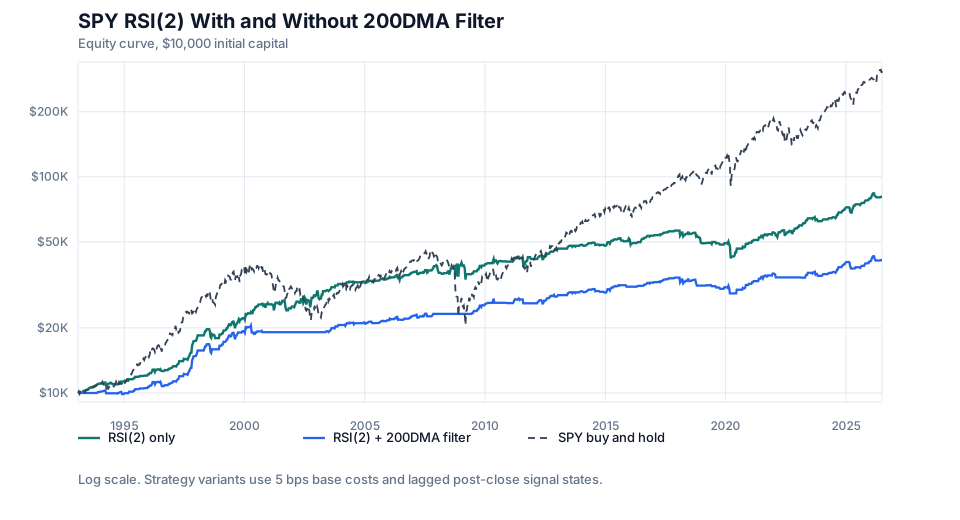
At 5 bps per position change, RSI(2) only finished at $80,712 with a -30.41% max drawdown. RSI(2) with the 200DMA filter finished at $41,195 with a -15.55% max drawdown. I read that as a risk-shaping tradeoff, not a clean improvement.
Why RSI(2)
RSI(2) is a very short-horizon oscillator. Here it is used as a mean reversion signal: low RSI marks a possible oversold entry, and high RSI marks an exit.
That makes it a useful contrast with the earlier moving-average studies. The 200DMA is slow and trend-oriented; RSI(2) is fast and reactive. This test asks what happens when the slow filter is placed around the fast signal.
Method
The backtest compares two variants:
| Variant | Entry condition | Exit condition |
|---|---|---|
| RSI(2) only | RSI(2) < 10 | RSI(2) > 70 |
| RSI(2) + 200DMA filter | RSI(2) < 10 and adjusted close > SMA200 | RSI(2) > 70 or adjusted close < SMA200 |
Both variants use a state machine. If the strategy is in cash and the raw entry condition is true, the post-close state becomes invested. If the strategy is invested and the raw exit condition is true, the post-close state becomes cash. Otherwise the previous state is carried forward.
The 200-day moving average is only a trend filter in the second variant. It does not create an entry by itself.
Data
| Field | Value |
|---|---|
| Source | Yahoo Finance via yfinance |
| Ticker | SPY |
| Price series | Adjusted close |
| Start date | 1993-01-29 |
| End date | 2026-07-02 |
| First valid RSI(2) date | 1993-02-02 |
| First valid SMA200 date | 1993-11-11 |
| Metric window | Includes indicator warmup period |
| Initial capital | $10,000 |
| Base transaction cost | 5 bps per position change |
| Cash return | 0% |
The script uses a local data/SPY.csv cache when present. Running python3 backtest.py --refresh-data replaces the cache with a fresh yfinance download.
RSI Calculation
RSI(2) is computed directly from adjusted-close differences. The code does not depend on TA-Lib.
For window n = 2:
delta[t] = adjusted_close[t] - adjusted_close[t - 1]
gain[t] = max(delta[t], 0)
loss[t] = max(-delta[t], 0)
The first valid average gain and loss are simple means of the first n daily gains and losses. After that, the script uses Wilder smoothing:
avg_gain[t] = (avg_gain[t - 1] * (n - 1) + gain[t]) / n
avg_loss[t] = (avg_loss[t - 1] * (n - 1) + loss[t]) / n
RSI[t] = 100 - 100 / (1 + avg_gain[t] / avg_loss[t])
If both average gain and average loss are zero, RSI is set to 50. If average loss is zero and average gain is positive, RSI is set to 100.
Signal Definition
The RSI-only variant is:
entry_signal[t] = RSI(2)[t] < 10
exit_signal[t] = RSI(2)[t] > 70
The filtered variant is:
entry_signal[t] = RSI(2)[t] < 10 and adjusted_close[t] > SMA200[t]
exit_signal[t] = RSI(2)[t] > 70 or adjusted_close[t] < SMA200[t]
The filtered variant cannot enter before the SMA200 exists. The first 199 trading days have no valid SMA200, so adjusted_close > SMA200 is false for entry purposes.
Execution and Cost Assumptions
This study uses the same close-to-close same-close approximation as the earlier SPY moving-average studies. A signal state updated after the close of day t-1 determines the modeled position for the close t-1 to close t return interval:
position[t] = signal_state[t - 1]The first row position is zero. This means the signal date’s close is not used to earn the same close-to-close return ending on that date.
The base case deducts 5 bps of portfolio equity when the position changes. The sensitivity table also shows 0 bps and 10 bps.
Results
The 5 bps base case shows a clear exposure difference. The RSI-only version was in SPY 20.88% of days. The filtered version was in SPY 12.42% of days.
| Metric | RSI(2) only | RSI(2) + 200DMA filter | SPY buy and hold |
|---|---|---|---|
| CAGR | 6.45% | 4.33% | 10.81% |
| Annualized volatility | 11.68% | 6.26% | 18.57% |
| Sharpe ratio, 0% rf | 0.59 | 0.71 | 0.65 |
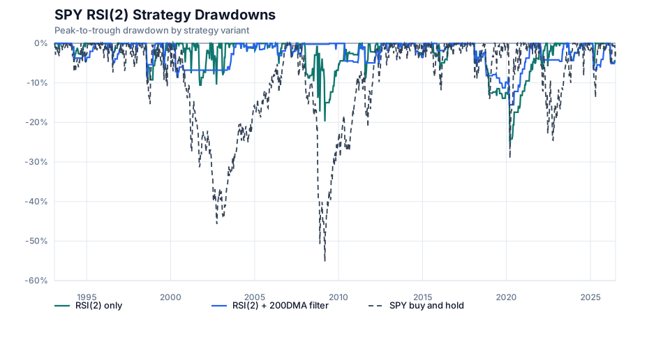
| Max drawdown | -30.41% | -15.55% | -55.19% |
| Calmar ratio | 0.21 | 0.28 | 0.20 |
| Time in market | 20.88% | 12.42% | 100.00% |
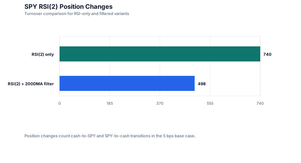
| Position changes | 740 | 498 | Initial buy only |
| Average holding days | 4.7 | 4.2 | - |
| Final equity | $80,712 | $41,195 | $308,867 |
Interpretation
The filter did what a filter often does: it removed exposure. Volatility fell from 11.68% to 6.26%, max drawdown improved from -30.41% to -15.55%, and position changes fell from 740 to 498.
The cost was opportunity cost. The RSI-only rule entered many oversold periods below the 200DMA. Some of those entries were early or uncomfortable, but some captured rebounds. The filtered version sat out those cases. In this sample, that reduced drawdown but also lowered final equity by roughly half relative to the unfiltered RSI rule.
I would not summarize this as the 200DMA filter improving the RSI(2) strategy in a broad sense. It improved some risk metrics and worsened the compounding metrics in the CSV output.
Robustness Checks
The table below reruns both variants at 0, 5, and 10 bps per position change.
| Variant | Cost | CAGR | Sharpe | Max drawdown | Position changes | Final equity |
|---|---|---|---|---|---|---|
| RSI(2) only | 0 bps | 7.63% | 0.69 | -28.93% | 740 | $116,823 |
| RSI(2) only | 5 bps | 6.45% | 0.59 | -30.41% | 740 | $80,712 |
| RSI(2) only | 10 bps | 5.28% | 0.50 | -31.86% | 740 | $55,752 |
| RSI(2) + 200DMA filter | 0 bps | 5.11% | 0.83 | -14.06% | 498 | $52,834 |
| RSI(2) + 200DMA filter | 5 bps | 4.33% | 0.71 | -15.55% | 498 | $41,195 |
| RSI(2) + 200DMA filter | 10 bps | 3.55% | 0.59 | -17.02% | 498 | $32,115 |
The cost sensitivity is material because RSI(2) is active. Even with the trend filter, 498 position changes left visible cost drag between the 0 bps and 10 bps rows.
Comparison with the 200DMA Studies
This RSI test is not just another version of the 200DMA trend-following studies. It uses the 200DMA as a gate around a short-term mean reversion rule.
| Study variant | CAGR | Max drawdown | Time in market | Position changes | Final equity |
|---|---|---|---|---|---|
| RSI(2) + 200DMA filter | 4.33% | -15.55% | 12.42% | 498 | $41,195 |
| Daily 200DMA | 8.08% | -29.42% | 75.35% | 215 | $134,111 |
| Golden cross 50/200 | 9.64% | -33.72% | 75.15% | 31 | $216,554 |
| Month-end 200DMA | 9.88% | -25.73% | 75.63% | 43 | $232,962 |
| SPY buy and hold | 10.81% | -55.19% | 100.00% | Initial buy only | $308,867 |
The filtered RSI strategy had the lowest drawdown in that table, but also the lowest final equity. It was out of the market most of the time. That makes it a different exposure profile from the 200DMA studies, not a simple upgrade to them.
Limitations
The execution model is still a simplification. A same-close close-to-close approximation keeps the adjusted close return series internally consistent, but it is not a next-open fill model.
Cash earns 0%, which understates cash-period returns when short-term rates are high. Taxes, account constraints, bid/ask spreads, market impact, and intraday order behavior are not modeled.
The thresholds are fixed at RSI(2) below 10 for entry and above 70 for exit. This study does not search over parameters. Different RSI windows, thresholds, assets, cash proxies, or execution assumptions could change the result.
Reproducibility
Run the study from the research repository:
cd studies/spy-rsi-2-200-day-moving-average-filter
pip install -r requirements.txt
python3 -B -m unittest discover -s . -p "test_*.py"
python3 backtest.py
python3 plot.py
The generated files are:
| File | Purpose |
|---|---|
data/SPY.csv | Cached adjusted OHLCV from yfinance |
outputs/spy-rsi2-200dma-filter-summary.csv | Summary metrics for both variants and 0/5/10 bps cost scenarios |
outputs/spy-rsi2-200dma-filter-equity.csv | Base-case daily indicators, signals, positions, returns, costs, equity, and drawdowns |
outputs/spy-rsi2-200dma-filter-trades.csv | Base-case position-change log |
charts/spy-rsi2-200dma-filter-equity-curve.svg | Equity curve comparison |
charts/spy-rsi2-200dma-filter-drawdowns.svg | Drawdown comparison |
charts/spy-rsi2-200dma-filter-position-changes.svg | Position-change comparison |
Only the summary CSV and SVG charts are copied into this site. The full equity and trade CSVs are generated by the code above.
FAQ
What is RSI(2)?
RSI(2) is a two-period Relative Strength Index. In this study it is calculated from adjusted-close daily differences using Wilder smoothing. A low value marks a short-term oversold condition in the rule being tested.
Is the 200-day moving average used as a trend filter or an entry signal?
It is a trend filter. The filtered variant can enter only when RSI(2) is below 10 and adjusted close is above SMA200. Being above SMA200 by itself does not create an entry.
How is look-ahead bias avoided?
The code separates post-close signal state from modeled position. A state computed after close t becomes position[t + 1]. In the CSV this is implemented as Position = SignalState.shift(1).
Why compare RSI(2) with and without the 200DMA filter?
The comparison isolates the filter. The RSI thresholds, data, benchmark, cost assumptions, cash return, and execution approximation are the same for both variants.
Does the trend filter reduce drawdowns?
In this CSV output, yes. The 5 bps max drawdown improved from -30.41% for RSI(2) only to -15.55% with the 200DMA filter. That came with lower CAGR and lower final equity in the same run.
How are transaction costs modeled?
Costs are deducted as a fixed percentage of portfolio equity on position-change days. The base case uses 5 bps per change, with 0 bps and 10 bps sensitivity rows.
More notes
Monthly Contributions in SPY, QQQ, and ETF Portfolios
A reproducible monthly contribution backtest comparing SPY, QQQ, a 60/40 stock-bond portfolio, and a simple multi-asset ETF portfolio using adjusted-close data.
Monthly QQQ Contributions Through the Dot-Com Crash
A reproducible backtest of monthly QQQ contributions starting in 2000, compared with SPY contributions and QQQ's dot-com price recovery path.