
Quick Take
This is a US equity ETF rotation backtest, not a multi-asset allocation test. The script rotates only among SPY, QQQ, and older sector ETFs; it does not include bonds, gold, commodities, REITs, or international equities.
Once a month, the script ranks the US equity ETF universe by trailing 126-trading-day adjusted-close return and then holds either Top 1 momentum or Top 3 momentum after a one-trading-day lag.
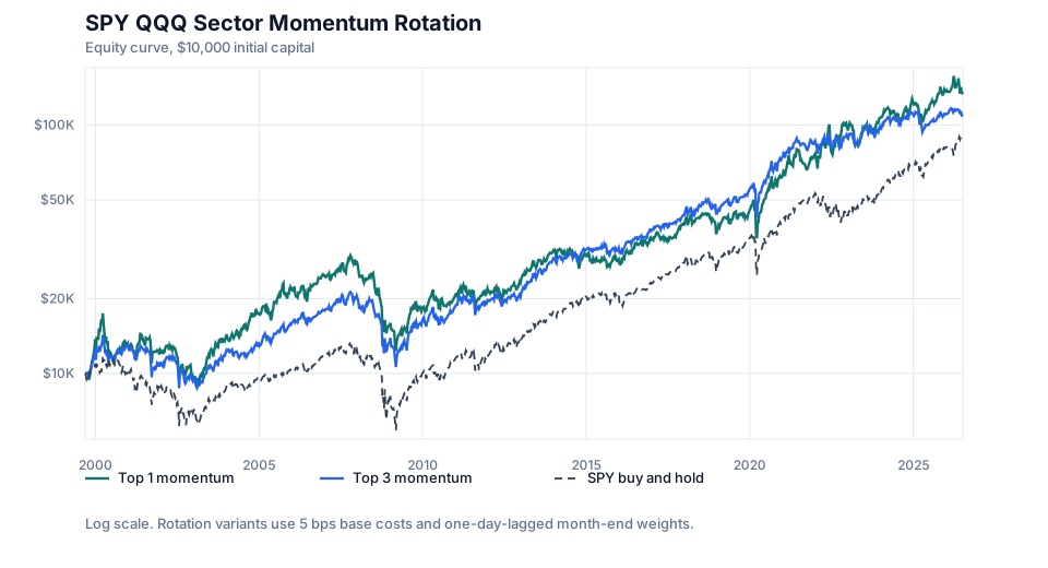
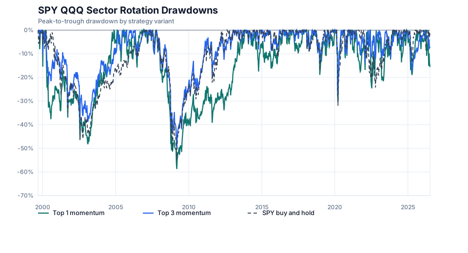
In the 5 bps base case, Top 1 momentum finished at $133,147 with a -58.76% max drawdown. Top 3 momentum finished at $110,285 with a -50.16% max drawdown. SPY buy and hold finished at $88,980 with a -55.19% max drawdown over the same strategy window.
My read is that US equity rotation changed the path, but not in a simple one-way way. Top 1 momentum had the higher ending value; Top 3 momentum was more diversified within equities and had the shallower drawdown.
Why ETF Rotation
Single-asset timing studies ask whether one rule can step in and out of SPY. This test asks whether monthly relative strength among SPY, QQQ, and sector ETFs changes the return and drawdown path versus simply holding SPY.
It is a relative-strength test inside US equities. After the first valid month-end signal, the main decision is which equity ETF or ETFs to hold.
Method
The backtest compares two monthly US equity ETF momentum strategy variants:
| Variant | Rule |
|---|---|
| Top 1 momentum | Hold the highest-ranked ETF by trailing 126-trading-day adjusted-close return |
| Top 3 momentum | Hold the highest-ranked ETFs by the same measure, equal weighted |
The benchmark is SPY buy and hold over the same strategy window. Initial capital is $10,000. Cash return is 0.00%.
US Equity ETF Universe
The universe has 11 ETFs:
| ETF | Role |
|---|---|
| SPY | S&P 500 ETF, broad large-cap benchmark |
| QQQ | Nasdaq 100 ETF, growth and technology-heavy exposure |
| XLK | Technology sector ETF |
| XLF | Financial sector ETF |
| XLV | Health Care sector ETF |
| XLY | Consumer Discretionary sector ETF |
| XLI | Industrial sector ETF |
| XLP | Consumer Staples sector ETF |
| XLE | Energy sector ETF |
| XLU | Utilities sector ETF |
| XLB | Materials sector ETF |
A separate multi-asset rotation study would use a different universe.
XLC and XLRE are excluded for this run because their histories are shorter than the older sector SPDR ETFs. The point of this sample is to keep a longer overlapping history across the selected US equity ETF universe.
Data
| Field | Value |
|---|---|
| Source | Yahoo Finance via yfinance |
| ETF universe | SPY QQQ XLK XLF XLV XLY XLI XLP XLE XLU XLB |
| Price series | Adjusted close |
| Start date | 1999-09-08 |
| End date | 2026-07-07 |
| Momentum lookback | 126 trading days |
| Rebalance frequency | Monthly, last available trading day |
| Initial capital | $10,000 |
| Base transaction cost | 5 bps per dollar traded / turnover |
| Cash return | 0.00% |
The script uses a local data/{TICKER}.csv cache when present. Each ETF has its own cache file.
Momentum Calculation
Momentum is the trailing 126-trading-day adjusted-close return:
momentum[t] = adjusted_close[t] / adjusted_close[t - lookback] - 1Why 126 trading days? The study uses 126 trading days as a practical approximation for six months, based on the common 252-trading-day convention for one US trading year. Half of 252 is 126, so the lookback is a simple half-year trading-day approximation.
It is not the same as measuring performance from one calendar month-end to another. The choice keeps the lookback length consistent across all dates, and it is a fixed assumption rather than an optimized parameter. A future robustness study could compare 63-, 126-, and 252-day momentum windows, or use strict calendar month-end returns.
Rebalance and Execution Timing
The ranking is calculated only on the last available trading day of each calendar month. The target weights are set after that close and then shifted forward before returns are applied:
actual_weights = target_weights.shift(1)That means a signal computed at a month-end close is not used for the close-to-close return ending on the same date. The first row of actual weights is zero.
Transaction Cost Assumptions
Costs are turnover-based:
turnover[t] = sum(abs(weights[t] - weights[t - 1]))
trading_cost[t] = turnover[t] * cost_bps / 10000
This matters for ETF rotation. Moving from cash into a fully invested ETF position has lower turnover than fully switching from one ETF to another ETF. The summary CSV includes 0 bps, 5 bps, 10 bps cost scenarios.
Results
The base-case results are:
| Metric | Top 1 momentum | Top 3 momentum | SPY buy and hold |
|---|---|---|---|
| CAGR | 10.13% | 9.36% | 8.49% |
| Annualized volatility | 24.07% | 19.10% | 19.27% |
| Sharpe ratio, 0% rf | 0.52 | 0.57 | 0.52 |
| Max drawdown | -58.76% | -50.16% | -55.19% |
| Calmar ratio | 0.17 | 0.19 | 0.15 |
| Time in market | 99.75% | 99.75% | Fully invested |
| Rebalance count | 138 | 223 | Initial buy only |
| Total turnover | 275.0 | 193.0 | Initial buy only |
| Average number of holdings | 1.00 | 2.99 | SPY only |
| Final equity | $133,147 | $110,285 | $88,980 |
Interpretation
The Top 1 rule is concentrated. That helped ending wealth in this sample, but it also produced the deepest drawdown among the two rotation variants. That should not be surprising: Top 1 can hold a single equity or equity-sector ETF through a bad period.
The Top 3 rule spread exposure across the highest-ranked ETFs, which reduced the worst drawdown versus Top 1 but also ended lower. Sector rotation can diversify within equities, but broad equity risk remains.
The benchmark comparison is useful, but it needs that equity-only context. SPY buy and hold had a strong final value in the same window. The rotation rules reshaped sector and style exposure, while still leaving the portfolio exposed to broad equity bear markets.
Robustness Checks
The table below reruns both rotation variants at the CSV cost scenarios.
| Variant | Cost | CAGR | Sharpe | Max drawdown | Total turnover | Final equity |
|---|---|---|---|---|---|---|
| Top 1 momentum | 0 bps | 10.70% | 0.54 | -58.35% | 275.0 | $152,756 |
| Top 1 momentum | 5 bps | 10.13% | 0.52 | -58.76% | 275.0 | $133,147 |
| Top 1 momentum | 10 bps | 9.57% | 0.50 | -59.17% | 275.0 | $116,039 |
| Top 3 momentum | 0 bps | 9.75% | 0.58 | -49.89% | 193.0 | $121,427 |
| Top 3 momentum | 5 bps | 9.36% | 0.57 | -50.16% | 193.0 | $110,285 |
| Top 3 momentum | 10 bps | 8.97% | 0.55 | -50.42% | 193.0 | $100,160 |
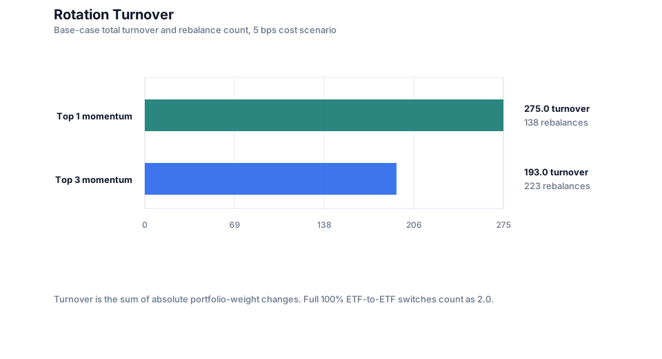
The cost sensitivity is larger for the more concentrated rule because full ETF-to-ETF switches can produce more turnover. The Top 3 rule still trades, but partial equal-weight changes make the cost drag less abrupt.
The momentum window itself is not optimized in this note. The 126-trading-day lookback is the fixed six-month approximation used for the main run.
Comparison with Single-Asset SPY Studies
This rotation test is not a replacement for the single-asset SPY studies. It asks a different question: cross-sectional leadership among ETFs, not whether SPY itself is above a moving average or in an RSI state.
| Study variant | CAGR | Max drawdown | Time in market | Final equity |
|---|---|---|---|---|
| US equity ETF rotation Top 1 | 10.13% | -58.76% | 99.75% | $133,147 |
| US equity ETF rotation Top 3 | 9.36% | -50.16% | 99.75% | $110,285 |
| Daily SPY 200DMA | 8.08% | -29.42% | 75.35% | $134,111 |
| Golden cross 50/200 | 9.64% | -33.72% | 75.15% | $216,554 |
| Month-end SPY 200DMA | 9.88% | -25.73% | 75.63% | $232,962 |
| RSI(2) + 200DMA filter | 4.33% | -15.55% | 12.42% | $41,195 |
| SPY buy and hold | 8.49% | -55.19% | Fully invested | $88,980 |
Be careful with that table: the SPY-only studies start on a different data window, while this rotation study starts only after every included ETF has overlapping data and a valid momentum lookback.
Limitations
The execution model is simplified. It uses adjusted close returns and a same-close close-to-close approximation, not strict next-open fills. Cash earns 0.00%; taxes, spreads, market impact, fund changes, and intraday execution are not modeled.
The universe is equity-only. No Treasury ETF, gold ETF, commodity ETF, REIT ETF, or international equity ETF is included, so broad equity bear markets can still produce large drawdowns.
XLC and XLRE are excluded because their shorter histories would shorten the common sample. The 126-trading-day lookback is also fixed, not optimized. Natural follow-ups would test other momentum windows or a separate multi-asset universe such as SPY, TLT or IEF, GLD, DBC or PDBC, VNQ, EFA, and EEM.
Reproducibility
Run the study from the research repository:
cd studies/spy-qqq-sector-momentum-rotation-backtest
pip install -r requirements.txt
python3 -B -m unittest discover -s . -p "test_*.py"
python3 backtest.py
python3 plot.py
The generated files are:
| File | Purpose |
|---|---|
data/{TICKER}.csv | Cached adjusted OHLCV from yfinance for each ETF |
outputs/spy-qqq-sector-momentum-rotation-summary.csv | Summary metrics for both variants and cost scenarios |
outputs/spy-qqq-sector-momentum-rotation-equity.csv | Base-case daily returns, costs, turnover, equity, drawdowns, and ETF weights |
outputs/spy-qqq-sector-momentum-rotation-trades.csv | Base-case rebalance log |
charts/spy-qqq-sector-momentum-rotation-equity-curve.svg | Equity curve comparison |
charts/spy-qqq-sector-momentum-rotation-drawdowns.svg | Drawdown comparison |
charts/spy-qqq-sector-momentum-rotation-turnover.svg | Turnover and rebalance-count comparison |
Only the summary CSV and SVG charts are copied into this site. The full equity and trade CSVs are generated by the code above.
FAQ
What is an ETF momentum rotation strategy?
It ranks ETFs by recent relative performance and rotates into the strongest ETF or ETFs on a set schedule. Here, the schedule is monthly.
Is this a multi-asset momentum strategy?
No. This is a US equity ETF and sector rotation test. It does not include bonds, gold, commodities, REITs, or international equities.
Which ETFs are included?
The included ETFs are SPY QQQ XLK XLF XLV XLY XLI XLP XLE XLU XLB. XLC and XLRE are excluded because their shorter histories would shorten the common sample.
How is momentum calculated?
Momentum is adjusted_close[t] / adjusted_close[t - {lookback}] - 1. The 126-trading-day lookback is a practical six-month approximation based on the common 252-trading-day year convention, not an optimized parameter or strict calendar-month return.
Why not include bonds, gold, or commodities?
That would answer a different question and change the universe being tested. A stocks, bonds, gold, commodities, REITs, and international equities rotation model should be tested as a separate multi-asset study.
How is look-ahead bias avoided?
Month-end target weights are shifted by one trading day before returns are applied, so the signal date’s close is not used to earn the same close-to-close return.
How are transaction costs modeled?
Costs are based on turnover: sum(abs(weights[t] - weights[t - 1])) * cost_bps / 10000. The summary CSV includes 0 bps, 5 bps, 10 bps rows.
Does Top 1 or Top 3 rotation have lower drawdown?
In the base-case CSV, Top 3 momentum has the lower max drawdown at -50.16% versus -58.76% for Top 1 momentum. Because the universe is equity-only, broad equity bear markets can still produce large drawdowns.
How does this compare with SPY buy and hold?
In the same rotation-study window, SPY buy and hold finished at $88,980 with a -55.19% max drawdown. The rotation variants changed the return and drawdown path rather than creating a one-way improvement across every metric.
More notes
Monthly Contributions in SPY, QQQ, and ETF Portfolios
A reproducible monthly contribution backtest comparing SPY, QQQ, a 60/40 stock-bond portfolio, and a simple multi-asset ETF portfolio using adjusted-close data.
Monthly QQQ Contributions Through the Dot-Com Crash
A reproducible backtest of monthly QQQ contributions starting in 2000, compared with SPY contributions and QQQ's dot-com price recovery path.